Fast, Cheap, and Competitive: Reservoir Computing for Predictive Maintenance
Any business running instrumented mechanical equipment — turbines, pumps, compressors, motors, manufacturing lines — faces the same tradeoff: schedule maintenance too early and you scrap good parts; too late and you risk unplanned downtime. The prediction problem behind that decision has the same shape everywhere: estimate how much useful life is left from a sensor time series. Aircraft engines are just an unusually well-instrumented, well-benchmarked example of it.
I built code-pipelines and compared three approaches to that problem on NASA’s C-MAPSS FD004 dataset, deliberately choosing the hardest of the four standard subsets, which combines 6 operating conditions and 2 simultaneous fault modes. I picked it as a rigorous public proving ground, not because aircraft specifically were the point.
A classical Echo State Network, fast and cheap enough to matter
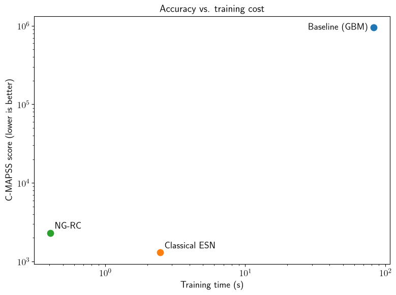
A classical Echo State Network (ESN) is a reservoir computing model: a fixed random recurrent network, driven directly by raw sensor history, with only a linear readout trained on top. No backpropagation, no GPU, nothing resembling a deep-learning training loop. It trains in 2.47 seconds on a desktop CPU (AMD Ryzen 7 8700G), roughly 33x faster than a properly tuned, vanilla gradient-boosting baseline (82.54s) on the same task. Published deep-learning approaches on this exact dataset need a GPU and still take longer: one reports 32.96s on an NVIDIA T4, and its own authors note GPU acceleration cut their training time by ~93% versus CPU, meaning a CPU-only run would land in the hundreds of seconds. This ESN needs neither the GPU nor anywhere near that time.
Speed alone doesn’t matter if accuracy suffers for it. On the C-MAPSS score, the benchmark’s own metric, this ESN is nearly three orders of magnitude better than gradient boosting (1,298.9 vs. 953,273.7), and is competitive with considerably heavier published approaches on the same dataset — beating some outright, trailing the best of them. Sorted by C-MAPSS score:
| Approach | C-MAPSS score | RMSE | Training cost |
|---|---|---|---|
| TCN-RC (Verghese et al., 2026)* | 446.73 | 17.97 | 32.96s, GPU |
| This ESN | 1,298.9 | 16.38 | 2.47s, CPU only |
| MLEAN (Li et al., 2025) | 1,370.0 | 16.89 | — |
| Hybrid Ensemble: DeepSSM+CatBoost+LightGBM (Vaishnavi et al., 2026) | 1,760.1 | 17.09 | — |
| LightGBM (Özcan, 2025) | 25,970 | 11.70 | — |
| Ensemble (LightGBM+CatBoost+GB) | 38,690 | 14.12 | — |
*RUL clipping protocol not stated; the paper’s own RUL formula includes no cap term, unlike every other entry here (clipped at 125).
This ESN is better than MLEAN and the DeepSSM/CatBoost/LightGBM ensemble on score, with an architecture simpler than either: a fixed random reservoir and a linear readout, nothing trained end-to-end. TCN-RC scores better still, but it needs a GPU and 32.96s to get there; this ESN’s CPU-only training cost is a real advantage in a total cost-of-ownership picture, separate from where it lands on the leaderboard.
The C-MAPSS score matters more than RMSE for this comparison because it’s the benchmark’s own asymmetric metric: it penalizes late, overestimating predictions far more heavily than early ones, since underestimating how much life is left is the costlier mistake in practice — miss it and equipment fails before anyone expected it to. By RMSE alone, gradient boosting (58.17) looks merely 3-4x worse than the reservoir models; by score, it’s in a different league entirely. That gap is what “competitive” is measured against here, not a simple ratio.
Another RC model: NG-RC
I also tuned NG-RC (next-generation reservoir computing), a newer variant with no random reservoir at all: just delay-embedded sensor history, a polynomial feature expansion, and a linear readout. To the best of my knowledge, there is no prior published application of it to this dataset or problem.
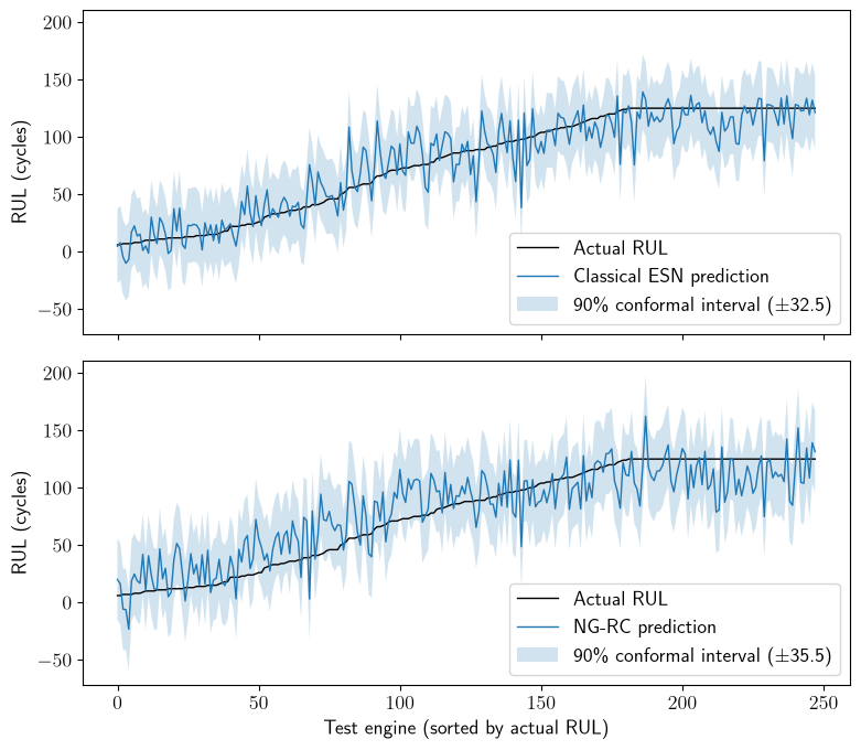
NG-RC trains even faster than ESN (0.41s vs. 2.47s) and is fully deterministic, giving the same answer every run. ESN’s own C-MAPSS score swings by more than 2.5x across different random seeds (995.4 to 2,533.7 across 100 seeds). That’s not a deployment problem — a trained, seed-fixed ESN is just as reproducible as NG-RC once shipped. It’s an extra training-time cost: a blind seed draw isn’t guaranteed to give the best prediction. Finding a good candidate to deploy takes trying several seeds first. What NG-RC doesn’t do on this dataset is match ESN’s accuracy: RMSE 21.08 and score 2,315.3, both worse than ESN’s. Its case holds up where skipping that seed-search step or very frequent retraining matter more than a few points of score — a real deployment scenario, just not the headline here.
Full methodology, and what didn’t work
Full methodology, the complete tuning history, additional diagnostic investigations, and the literature comparison are in the project repo — including the parts that didn’t pan out (kfold validation of NGRC, a LightGBM swap).
github.com/shail-kumar/reservoir-computing-predictive-maintenance